Notes on Controllable Text Generation
Recently, I have come across the Controllable Text Generation paper. This paper aims at generating natural language sentences, whose attributes are dynamically controlled by representations with designated semantics. I liked this paper a lot. And if you haven’t read it yet, go ahead and do it now. Alright, assuming that you have just read it, are you confused as I was regarding “efficient collaborative learning of generator and discriminator”, “efficient mutual bootstrapping” or “explicit enforcement of the independence property”? I believe that there is a more rigorous way to get the same loss function that is discussed in the paper. So, if you are wondering how to do that, you are welcome to read these notes.
Outline
- Short story that I would like to use throughout these notes
- Directed graphical model for text generation
- A couple of words regarding variational autoencoder
- A couple of thoughts regarding mutual information
- Derivation of lower bound of mutual information
- Discussion of some VAE issues
- Some comments on Controllable Text Generation paper
Short story
Let me start with a short story that I would like to use throughout this post. I remember how during my school literature classes teacher always asked pupils about the main idea of a novel. “What message 📜 is he or she trying to communicate?” - The teacher was constantly asking. We often needed to figure out the author’s most important points and provide the pieces of evidence contained in the text 📖. The teacher always encouraged us to come up with more than one theory why the book had been written. Once in a while, someone gave a very unexpected interpretation of the story. In such situations, the teacher usually wasn’t very persuaded and replied that author was a rather “crazy” person but not that “crazy,” or he or she couldn’t think of X because at that time there wasn’t any X.
 Every now and then, we had to write an essay on a given topic. I can’t say that it was a very pleasant experience for me, but one time I got soaked myself in the task and wrote a very solid essay. I thought it would be a masterpiece, the punctuation and spelling were correct, the grammar was top notch. Even my teacher found it quite startling. The language was very fluent, and everything in that essay made a lot of sense. The only problem was it was completely off topic. I got a bad mark that day. I remember I was a little bit disappointed about that. In hindsight, I can say I would not have been so upset if I realized that during our literature classes we had been optimizing:
- a variational lower bound of marginal likelihood of the generative model for novels with latent themes
- a variational lower bound of mutual information between novels and themes
Graphical model
 There are already enough well-written high-quality explanations of variational autoencoders and variational inference in general. I am not aiming to give yet another explanation. I would rather like to use the next two sections to establish notation and to make sure that we are on the same page. If you are already familiar with VAE, you can skip and jump to the Mutual Information section.
We consider a directed graphical model for generating a novel \(x\) 📖 with a latent theme \(z\) 📜. Let’s use the same model for generating novel given a topic \(p(📖\vert📜)\) as in the Generating Sentences from a Continuous Space paper. More specifically, it is an LSTM recurrent neural network where the first hidden state is initialized with \(z\): 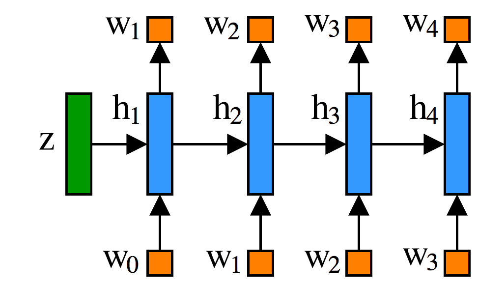 Let’s pause for a second and think what it means in terms of the described short story. On the figure above, you can see the model of the pupil who wants to write a book \(x\) 📖 given a topic \(z\) 📜. Variable \(h_t\) corresponds to the state of mind after reading \(t\) words. The good pupil is the one who assigns the high probability to the written books (training data). No one really knows what author wanted to tell. That is why we have to consider all possible human thoughts (topics) to get the probability of a book \(p(📖)=\int (p(📖\vert📜)d📜\). So, now the tough question arises: how to evaluate the marginal likelihood of the data? Typically, there is no analytical expression for the integral, even for such a simple model as shown in the figure.
Watch out! Evaluating marginal likelihood \(p(x)\) is hard.
Alright, if we can’t integrate it analytically, let’s estimate it using Monte Carlo method. One of the possible estimators and naïvest one is \(\frac{1}{K}\sum_{k=1}^{K}p(x\vert z_k)\) where \(z_k\) is a sample from \(p(z)\). Although it is unbiased, it can have very high variance especially in models where most latent configurations can’t explain a given observation well. In terms of our story, it is the same as if the teacher randomly gives pupils a topic and asks them to evaluate the probability of the book given this topic. Of course, most of the provided topics will not have any relation with the book, so most of the time the probability is going to be hugely underestimated.
Watch out! Naïve Monte Carlo estimator \(\frac{1}{K}\sum_{k=1}^{K}p(x\vert z_k)\) can have high variance.
But why does the teacher think that this kind of graphical model for the books even makes sense in the first place? I believe that it does. Typically, the dimensionality of the variable \(z\) is much much smaller than the dimensionality of the variable \(x\). And if you can perform inference over latent variable \(p(z\vert x)\) instead of learning a book by heart, you can just remember inferred \(z\) (compressed book). And when you need details, you can use your generative model \(p(x\vert z)\) to reconstruct book back. It is very convenient, it will free a lot of space in your head. Hence, you can read even more. Also, if you choose an appropriate structure for \(z\), so that you can easily compare two values, you can compute the similarity between two books pretty easily without going trough both of them and trying to compare everything word by word. This approach is pretty handy. But the problem is the same as with marginal likelihood: there is no analytical solution for \(p(z\vert x)\) and naïve Monte Carlo estimators will have high variance. So, as you can guess, the answer for this problem is variational autoencoder.
Watch out! Evaluating posterior distribution \(p(z \vert x)\) is hard.
Variational autoencoder
Variational autoencoder is a latent variable model equiped with an inference network. As we already know, it is not straigforward to evaluate marginal likelihood. So, it would not be easier to maximize it. Instead, we will use its lower bound. \[p(x) = \int p(x\vert z)p(z)dz = \int p(x\vert z)p(z)\frac{q(z\vert x)}{q(z\vert x)}dz = \int q(z\vert x)p(x\vert z)\frac{p(z)}{q(z\vert x)}dz\] Using Jensen’s inequality: \[\log{p(x)} \ge \int q(z\vert x)\log{\left(p(x\vert z)\frac{p(z)}{q(z\vert x)}\right)}dz = \int q(z\vert x)\log{p(x\vert z)}dz - \int q(z\vert x)\log{\frac{q(z\vert x)}{p(z)}}dz\] Finally, we have: \[\log{p(x)} \ge \mathbb{E}_{q(z\vert x)}[\log{p(x\vert z)}] -D_{KL}\left(q(z\vert x)\|p(z)\right) = \mathcal{L}(x)\] By maximizing lower bound \(\mathcal{L}(x)\), we will also maximize the marginal likelihood \(\log{p(x)}\). And, in the end, the value of marginal likelihood will be at least as large as the value of lower bound. The lower bound contains approximate posterior distribution \(q(z\vert x)\). It has such name because, as you already guessed, it is an approximation of the true posterior. By keeping parameters of \(p(x\vert z)\) fixed and optimizing the lower bound, you will be eventually minimizing \(D_{KL}\left(q(z\vert x)\|p(z\vert x)\right)\). Commonly \(q(z\vert x)\) belongs to the family of distributions that could be reparametrized. So, eventually, the gradients of the first term from the lower bound can be efficiently estimated with Monte Carlo methods (pathwise derivatives).
Surprisingly enough, the lower bound is exactly what pupils use to learn during literature classes.
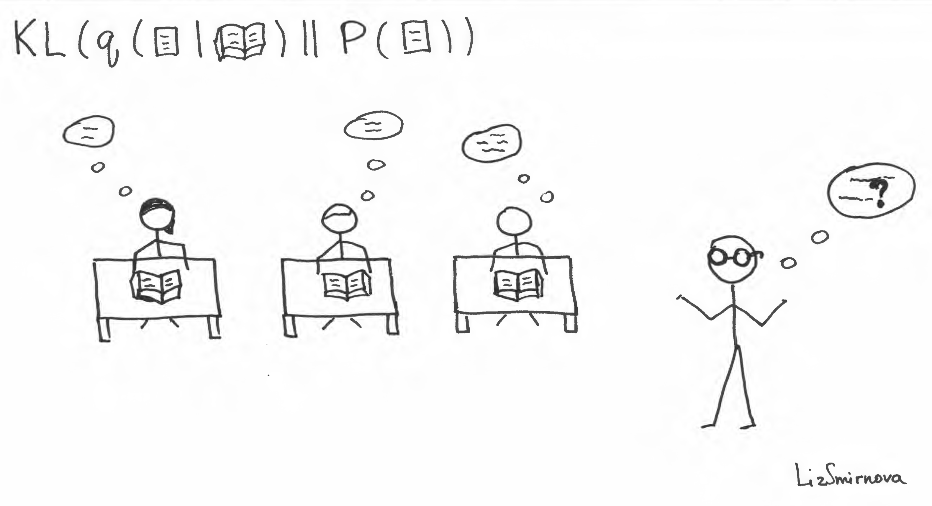
 At first, the teacher asks you to read a book and try to guess what authors had in mind while writing it. Making assumption about the theme is equivalent to sampling from \(q(📜\vert📖)\). Then, teacher is providing a feedback to the students about how probable is the guess with respect to all possible human thoughts \(p(\)📜\()\). At the same time, the teacher encourages the high entropy of \(q(📜\vert📖)\) by demanding several different interpretations from the class. To cut a long story short, the teacher evaluates the second term of the lower bound \(D_{KL}(q(📜\vert📖)\|p(📜))\).
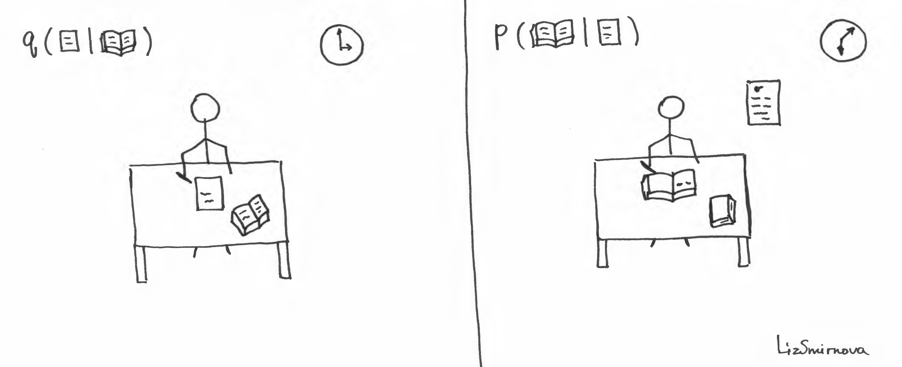
In terms of our story, reconstruction term corresponds to the process depicted in the image above. At first, you have to read a book and make your guess about the theme of the novel. Then, you have to write back the whole book using your guess. If you can provide a reasonable variety of guesses to make your teacher happy
At first, the teacher asks you to read a book and try to guess what authors had in mind while writing it. Making assumption about the theme is equivalent to sampling from \(q(📜\vert📖)\). Then, teacher is providing a feedback to the students about how probable is the guess with respect to all possible human thoughts \(p(\)📜\()\). At the same time, the teacher encourages the high entropy of \(q(📜\vert📖)\) by demanding several different interpretations from the class. To cut a long story short, the teacher evaluates the second term of the lower bound \(D_{KL}(q(📜\vert📖)\|p(📜))\).
In terms of our story, reconstruction term corresponds to the process depicted in the image above. At first, you have to read a book and make your guess about the theme of the novel. Then, you have to write back the whole book using your guess. If you can provide a reasonable variety of guesses to make your teacher happy
small \(D_{KL}(q(📜\vert📖)\|p(📜))\)
and you can write reasonable reconstruction of the text given your guess
big \(\mathbb{E}_{q(📜\vert📖)}[\log{p(📖\vert📜)}]\)
you will have a good lower bound and after all, you will be a good pupil, won’t you?
Mutual Information
If you think that a huge evidence lower bound is enough to be a good pupil, you are missing one important thing. Unfortunately, so was I in my school.
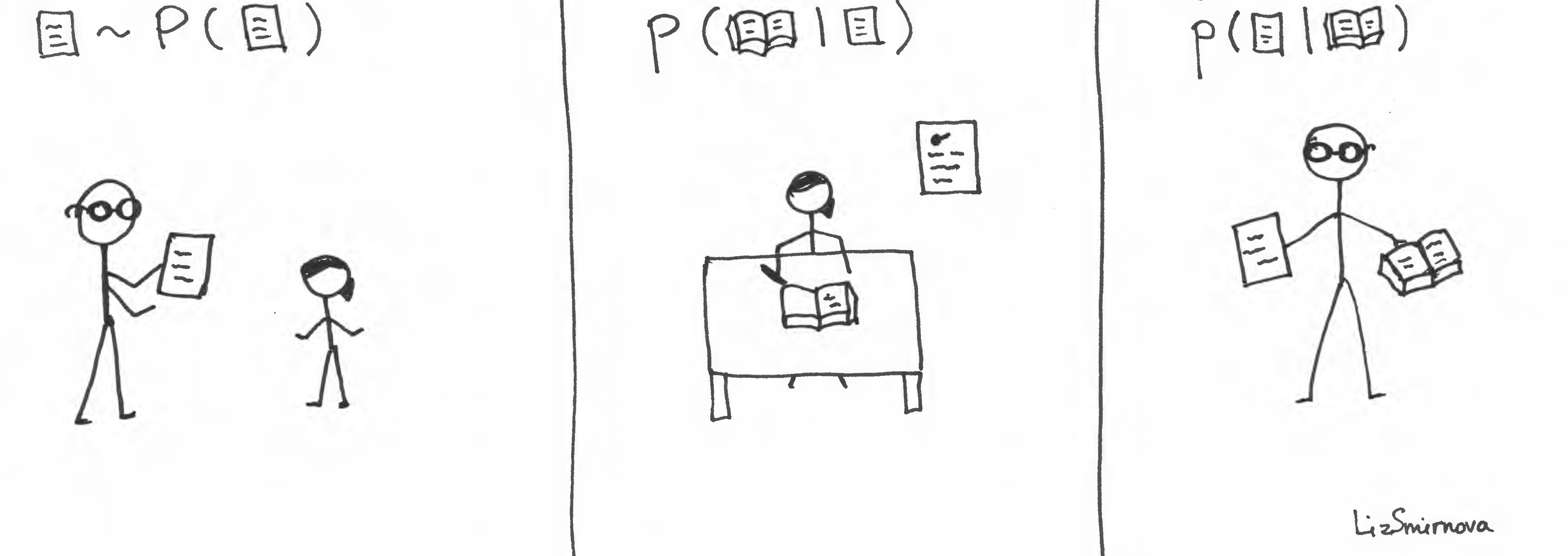 The key thing is writing essay on a given topic. At first, teacher has to give you a sample from \(p(📜)\). Then, you have to write an essay (sample from \(p(📖\vert📜)\)). Assuming that the teacher is a good teacher, then, he or she knows \(p(📜\vert📖)\). It measures how well your text corresponds to the topic. Hence, the mark for the homework will be proportional to this probability. Does this process remind you of something? It does remind me of the evaluation of mutual information:
\[I(x, z)=D_{KL}(p(x, z)\|p(x)p(z))=\int_z\int_x p(x,z) \log{\frac{p(x,z)}{p(x)p(z)}}dxdz\]
As you can see from the definition, the mutual information measures dependence between two variables. They are independent if and only if \(I(x,z)=0\)
The key thing is writing essay on a given topic. At first, teacher has to give you a sample from \(p(📜)\). Then, you have to write an essay (sample from \(p(📖\vert📜)\)). Assuming that the teacher is a good teacher, then, he or she knows \(p(📜\vert📖)\). It measures how well your text corresponds to the topic. Hence, the mark for the homework will be proportional to this probability. Does this process remind you of something? It does remind me of the evaluation of mutual information:
\[I(x, z)=D_{KL}(p(x, z)\|p(x)p(z))=\int_z\int_x p(x,z) \log{\frac{p(x,z)}{p(x)p(z)}}dxdz\]
As you can see from the definition, the mutual information measures dependence between two variables. They are independent if and only if \(I(x,z)=0\)
The first term corresponds exactly to described process of essay writing and evaluation. It measures how well you can preserve the topic in your text. Unfortunately, mutual information requires computation of intractable \(p(z\vert x)\).
Watch out! Evaluating mutual information \(I(x, z)\) is hard.
Variational lower bound for mutual information
As you can see, to be a really good pupil, you also have to have big mutual information \(I(📖,📜)\). But a pupil does not have access to the true posterior \(p(📜\vert📖)\). Is he or she doomed to fail? Of course, not. He or she can use their approximate posterior \(q(📜\vert📖)\) to evaluate an approximation to the true mutual information. More specifically:
\[\begin{aligned} I(x, z) - H(z) =\mathbb{E}_{p(z)}\left[\mathbb{E}_{p(x\vert z)}\log{p(z\vert x)}\right] \\ =\mathbb{E}_{p(z)}\left[\mathbb{E}_{p(x\vert z)}\log{\left(p(z\vert x)\frac{q(z\vert x)}{q(z\vert x)}\right)}\right] \\ =\mathbb{E}_{p(z)}\left[\mathbb{E}_{p(x\vert z)}\log{q(z\vert x)}\right] + \mathbb{E}_{p(z)}\left[\mathbb{E}_{p(x\vert z)}\log{\frac{p(z\vert x)}{q(z\vert x)}}\right] \\ =\mathbb{E}_{p(z)}\left[\mathbb{E}_{p(x\vert z)}\log{q(z\vert x)}\right] + \mathbb{E}_{p(x)}\left[\mathbb{E}_{p(z\vert x)}\log{\frac{p(z\vert x)}{q(z\vert x)}}\right] \\ =\mathbb{E}_{p(z)}\left[\mathbb{E}_{p(x\vert z)}\log{q(z\vert x)}\right] + \mathbb{E}_{p(x)}\left[D_{KL}\left(p(z\vert x)\|q(z\vert x)\right)\right] \end{aligned}\]Using the non-negativity property of KL-divergence, we can derive:
\[I(x, z)\ge\mathbb{E}_{p(z)}\left[\mathbb{E}_{p(x\vert z)}\log{q(z\vert x)}\right] + H(z)\]This result seems neat to me. We managed to boil down the essay-writing task to its core – evaluating mutual information. Also, there is a lower bound of it that is relatively cheap to evaluate. Unfortunately, the problem still remains. If we want to learn the model, we have to estimate the gradients of the mutual information lower bound. The root of the problem is a discrete nature of x. We can’t use pathwise derivatives because \(p(x\vert z)\) does not belong to any reparametrizable family. Especially, in the case of language, the score function estimator can have huge variance, and that makes learning impractical. Fortunately, due to recent development of deep learning, we can use low-variance biased gradient estimators that work in practice incredibly well. For example, I used the straight-through Gumbel-Softmax estimator in our recent work (Havrylov & Titov 2017) to learn language between two cooperative agents. By the way, it is not a coincidence that the loss function for communication looks very much like the variational lower bound of mutual information. After all, language is by definition something that we use to communicate information about the external world.
VAE issues
Now we have all building blocks to get a more rigorous explanation of the proposed model for controllable text generation. But before we dive into that, let me point out several important issues that arise while using VAE.
Mean field approximation
Typically, when using VAE, we make strong assumptions about the posterior distribution. For instance, the assumption that the posterior distribution is approximately factorial (mean field approximation). Within VAE framework, generator and inference network are trained jointly. So, they are encouraged to learn representations where these assumptions are satisfied (Importance Weighted Autoencoders, Variational inference for Monte Carlo objectives, Improving Variational Inference with Inverse Autoregressive Flow). In other words, training a powerful model using an insufficiently expressive variational posterior can cause the model to use only a small fraction of its capacity.
Using factorial variational posterior for VAE may make true posterior follow this constraint.
KL weight annealing hack
Another important feature of learning dynamic is that, at the start of training, the generator model \(p(x\vert z)\) is weak. That makes the state where \(q(z\vert x) \approx p(z) \) most attractive. In this state, inference network gradients have a relatively low signal-to-noise ratio, resulting in a stable equilibrium from which it is difficult to escape. The solution proposed in the Generating Sentences from a Continuous Space paper is to use an annealing for the weight of the \(D_{KL}(q(z\vert x)\|p(z))\) term, slowly increasing it from 0 to 1 over parameter updates. To be honest, I am not a big fan of this solution. It looks to me like a hack. I think we can do better.
How to deal with powerful \(p(x\vert z)\)
Alright, let’s say that now we are using this annealing trick. But did we manage to avoid the trivial \(q(z\vert x) \approx p(z)\) state? Not at all, when you have a very powerfull model for the likelihood \(p(x\vert z)\), most of the time you will encounter this trivial solution. Let’s illustrate it with my story example. It could seem that proposed model for the student is very simple, but in fact, LSTM RNN is a very powerful model that can fit your sequential data pretty well. Let’s say that pupil is in the phase of optimizing lower bound of the marginal log-likelihood. It consists of the expected reconstruction term and KL term. For optimizing the expected reconstruction term, a pupil has to read a book and make a guess about the theme and then he has to maximize the probability of reconstructing book back using this theme. It could seem that the reconstruction of the whole book is impossible. But, actually, this process does not look so complicated because on each time step you have access to the whole context that precedes the current word. The only thing that you have to predict on each time step is just one word. It is not surprising that pupil can be carried away by this process and can completely forget about the theme of the book. In the end, he or she can still write a decent essay, but it would be completely off topic (this is exactly what happened to me). To fight this problem, Bowman et. al proposed to make the generative model weaker by removing some or all of conditioning words during learning (taking away the book from pupil during reconstruction phase). But this solution also looks like a hack to me. I believe that using the mutual information in the loss function can solve this problem in a more principled way without making the generative model less expressive.
Using the variational lower bound of \(I(x, z)\) can solve the problem with trivial solution \(q(z\vert x) \approx p(z)\) for powerful likelihood \(p(x\vert z)\) in a more principled way.
Controllable text generation
Finally, we can get into the Controllable Text Generation paper. As you may already know, paper aims to generate natural language sentences, whose attributes are dynamically controlled by representations with designated semantics. They propose a “neural generative model which combines variational auto-encoders and holistic attribute discriminators for effective imposition of semantic structures.” I hope that after reading this post you can clearly see that “holistic attribute discriminator” is nothing more than approximate posterior inference network. And “collaborative learning of generator and discriminators” is just optimization of variational lower bound of mutual information. Despite the fact that both options sound mouthful, I am convinced that the second one is more mathematically rigorous, hence, useful.
One thing that I am still confused about is the claim: “proposed deep text generative model improves model interpretability by explicitly enforcing the constraints on independent attribute controls;”. They are saying that optimizing loss in equation 7 explicitly imposes independency constraint for posterior distributions. But if you look closely, you will see that it is just the variational lower bound of the mutual information between sentence \(x\) and latent code \(z\). I am not convinced that two posteriors \(p(z\vert x)\) and \(p(c\vert x)\) will be independent if you maximize mutual information \(I(x,z)\) and \(I(x,c)\). Using the definitions: \[I(z,c\vert x)=H(x,z) + H(x, c) - H(x,z,c)-H(x)\] \[H(x,z) = -I(x,z) + H(x) + H(z)\]
one can express the conditional mutual information through the mutual informaton:
\[\begin{aligned} I(z,c\vert x)=-I(x,z) -I(x,c) + H(x) + H(z) + H(c) - H(x,z,c) \\ =-I(x,z) -I(x,c) + H(x) - H(x\vert z,c) \end{aligned}\]Independency of posteriors is equvialent to \(I(z,c\vert x)=0\). To say the truth, I can’t see how maximizing mutual information \(I(x,z)\) and \(I(x,c)\) will make \(I(z,c\vert x)\) smaller. Even though, by doing so, you will lower down the first two terms in the equation but you will increase overall value for the last two. If you think I am missing something, please let me know. But for the time being, I think that saying that loss in the equation 7 in the paper explicitly encourages independency is not tehnically correct. Moreover, I am not sure that the column names for the table 2 are correct either. I would like to remind you of the VAE property that if you make independenсy assumptions in your approximate posterior network, it is probable that true posterior will also follow this constraint. It means that it is higly likely that both models with and without mutual information regularization have almost independent posteriors.
Another thing that totaly confused me was: “To avoid vanishingly small KL term in the VAE we use a KL term weight linearly annealing from 0 to 1 during training.” Why should you do that? If you have a variational lower bound of mutual information in your loss, it is already solving this problem in a more principled way. Why do you need to use this annealing hack?
Conclusion
In conclusion I would like to say one more time that I realy liked Controllable Text Generation paper. Even though, I am a little bit disappointed that authors have chosen (in my opinion) not the best way to explain the proposed model. If you think that I am missing something, feel free to let me know in the comments. I would be more than happy to discuss it.
But for now, I would like to conclude with this quote:
“…I thought my symbols were just as good, if not better, than the regular symbols - it doesn’t make any difference what symbols you use - but I discovered later that it does make a difference. Once when I was explaining something to another kid in high school, without thinking I started to make these symbols, and he said, “What the hell are those?” I realized then that if I’m going to talk to anybody else, I’ll have to use the standard symbols, so I eventually gave up my own symbols…”
Acknowledgements
I would like to thank Ivan Titov and Wilker Aziz for interesting discussions. Special thanks to Liza Smirnova for providing illustrations and proofreading the post.